用户分桶Spark任务性能调优

Posted Apr 8, 2026 Updated Apr 9, 2026

By Zhao Zhengyang

13 min read

用户分桶Spark任务性能调优

问题定义

有一张包含用户价值数据的Hive表user_pos_info，天级分区，具有以下字段：

partition_time：分区时间(yyyymmdd)
user_id：用户id
position_id：位置id
req_cnt：请求量
cost：价值

需求：按照用户的请求价值降序排序，并按请求量平均分为n个桶1~n（1桶价值最低、n桶价值最高），将结果以CSV格式输出到HDFS。用户的请求价值定义为：

cpr = sum(cost) / sum(req_cnt)

例如，对于以下示例数据

user_id	position_id	req_cnt	cost
1	2	60	120
1	4	20	80
2	2	40	0
2	3	50	20
3	1	20	100
4	3	60	90
5	1	20	5
5	2	25	25

假设桶数n = 3，则期望的分桶结果如下：

user_id	req_cnt	cost	cpr	bucket_id
3	20	100	5	3
1	80	200	2.5	3
4	60	90	1.5	2
5	45	30	0.86	2
2	90	20	0.18	1

其中3、2、1桶的请求量分别为100、105、90。

真实的数据量非常大，每个分区大小约2.1 TB，包含1380亿行、21亿个用户id，因此使用Spark框架进行计算。设定桶数n = 10。

方法1：全局排序

首先尝试最直接的全局排序方法：

计算用户的cpr。
使用窗口函数计算按cpr降序排序的累积请求量cum_req_cnt和总请求量total_req_cnt。
根据累积请求量比例计算桶id（前10%的用户属于10桶，10%~20%的用户属于9桶，以此类推）。

程序代码如下：

  
package com.example

import org.apache.spark.sql.expressions.Window
import org.apache.spark.sql.functions._
import org.apache.spark.sql.{DataFrame, SparkSession}

object UserBucket {
  def main(args: Array[String]): Unit = {
    val spark = SparkSession.builder().appName("UserBucket")
      .config("spark.sql.warehouse.dir", "...").enableHiveSupport()
      .getOrCreate()
    val userPosInfo = spark.table("user_pos_info")
      .filter(s"partition_time = ${args(0)}")

    val startTime = System.currentTimeMillis()
    println(s"calcUserBucket begins at $startTime")
    val bucketNum = 10
    val userBucket = calcUserBucket(userPosInfo, bucketNum).cache()
    userBucket.show()
    val endTime = System.currentTimeMillis()
    printf("calcUserBucket finished, cost %.2f seconds\n", (endTime - startTime) / 1000.0)

    userBucket.groupBy("bucket_id")
      .agg(count("user_id").as("user_cnt"),
        sum("req_cnt").as("req_cnt"),
        round(max("cpr"), 6).as("max_cpr"),
        round(min("cpr"), 6).as("min_cpr"))
      .orderBy(desc("bucket_id"))
      .show()

    userBucket.coalesce(200)
      .write
      .option("header", "true")
      .csv(args(1))
    spark.stop()
  }

  def calcUserBucket(userPosInfo: DataFrame, bucketNum: Int): DataFrame = {
    val userAgg = userPosInfo
      .groupBy("user_id")
      .agg(
        sum("req_cnt").as("req_cnt"),
        sum("cost").as("cost"))
      .filter("req_cnt > 0")
      .withColumn("cpr", expr("cost / req_cnt"))

    userAgg
      .withColumn("cum_req_cnt", sum("req_cnt").over(Window.orderBy(desc("cpr"))))
      .withColumn("total_req_cnt", sum("req_cnt").over(Window.partitionBy()))
      .withColumn("cum_ratio", expr("cum_req_cnt / total_req_cnt"))
      .withColumn("bucket_id", expr(s"$bucketNum + 1 - ceil(cum_ratio * $bucketNum)"))
  }
}

运行环境的Spark版本为3.3.1。任务使用250个executor*4核=1000核，并配置spark.sql.shuffle.partitions=2000。

根据程序输出可以验证结果的正确性：各桶的cpr依次递减，且请求量大致相等。

calcUserBucket finished, cost 15582.80 seconds
+---------+---------+------------+-----------+-----------+
|bucket_id| user_cnt|     req_cnt|    max_cpr|    min_cpr|
+---------+---------+------------+-----------+-----------+
|       10|330282810|272989032912|   1.0449E8|1409.544456|
|        9|182574435|272989105068|1409.544454| 808.294355|
|        8|136727249|272989067180|  808.29435| 566.414343|
|        7|132826920|272989071282|  566.41433| 403.616495|
|        6|119265555|272989045185| 403.616494| 291.970926|
|        5|108953339|272989093350| 291.970925| 208.354515|
|        4|100921986|272989065242| 208.354512| 141.902805|
|        3| 95360211|272989068781| 141.902804|  86.719478|
|        2| 93874745|272989047912|  86.719473|  39.304095|
|        1|808419721|272989095172|  39.304094|        0.0|
+---------+---------+------------+-----------+-----------+

但是任务共耗时6.1 h，不可接受，需要进行优化。从Spark UI可以看到各个阶段的耗时情况：

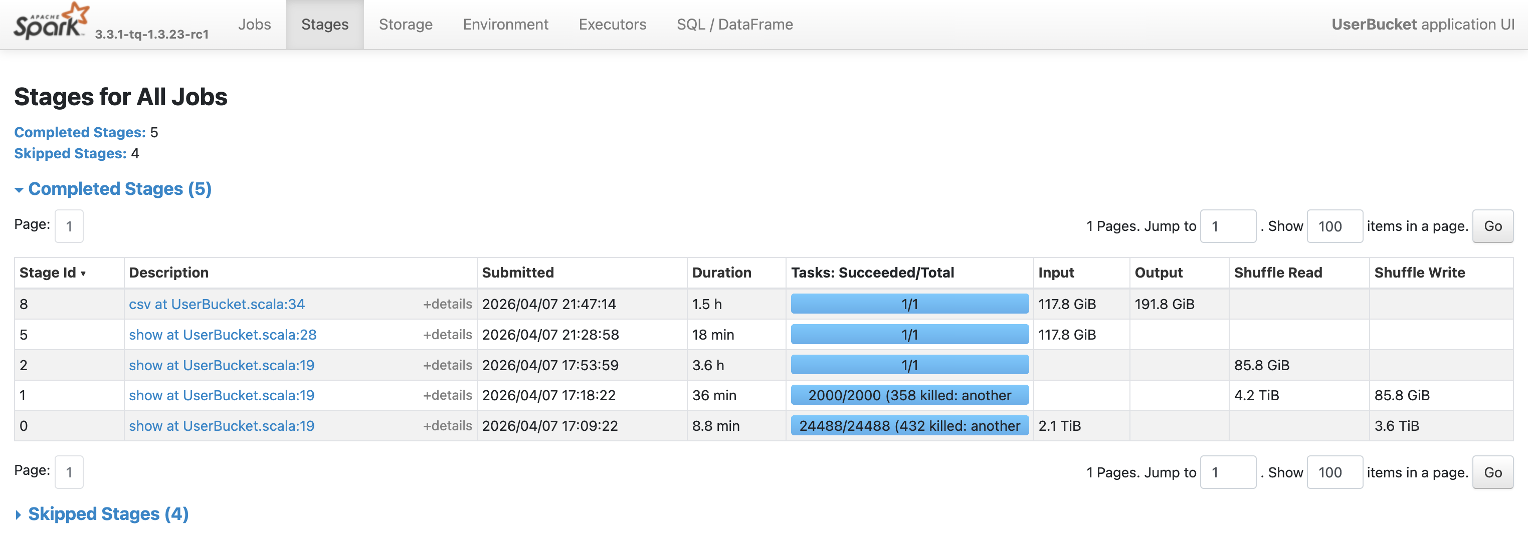
阶段	动作	并行度	耗时
0	读表，按用户id聚合，计算cpr	24488	8.8 min
1	窗口函数部分计算	2000	36 min
2	窗口函数最终计算，全局排序	1	3.6 h
8	输出CSV	1	1.5 h

可以看到，瓶颈在于Stage 2，需要在单个task中读取85.8 GB的shuffle数据并进行全局排序，导致计算过慢。

方法2：采样+近似分界点

分析问题要求可以发现，桶内用户的顺序并不重要，只需找到相邻桶的cpr分界点即可。例如，如果知道1和2桶的分界点是39.30，2和3桶的分界点是86.72，那么39.30 < cpr ≤ 86.72的用户都属于2桶。

因此，考虑对数据进行采样，在采样的数据上计算出所有桶的近似cpr分界点，之后根据这些分界点直接计算桶id：

  
CASE WHEN cpr > 1409.54 THEN 10
WHEN cpr > 808.29 THEN 9
...
WHEN cpr > 39.30 THEN 2
ELSE 1 END AS bucket_id

这样可以避免对全量数据进行排序，以牺牲一定的准确率为代价节省计算时间。修改后的代码如下（采样率取1/10000）：

  
def calcUserBucket(userPosInfo: DataFrame, bucketNum: Int): DataFrame = {
  val userAgg = userPosInfo
    .groupBy("user_id")
    .agg(
      sum("req_cnt").as("req_cnt"),
      sum("cost").as("cost"))
    .filter("req_cnt > 0")
    .withColumn("cpr", expr("cost / req_cnt"))
    .cache()

  val sampledUserBucket = userAgg
    .sample(0.0001)
    .withColumn("cum_req_cnt", sum("req_cnt").over(Window.orderBy(desc("cpr"))))
    .withColumn("total_req_cnt", sum("req_cnt").over(Window.partitionBy()))
    .withColumn("cum_ratio", expr("cum_req_cnt / total_req_cnt"))
    .withColumn("bucket_id", expr(s"$bucketNum + 1 - ceil(cum_ratio * $bucketNum)"))

  val cprBounds = sampledUserBucket
    .groupBy("bucket_id")
    .agg(min("cpr").as("min_cpr"))
    .collect()
    .map(r => (r.getAs[Long]("bucket_id"), r.getAs[Double]("min_cpr")))
    .sortBy(-_._2)

  val bucketConditions = cprBounds.tail
    .foldLeft(when(col("cpr") > cprBounds.head._2, cprBounds.head._1))(
      (c, t) => c.when(col("cpr") > t._2, t._1))
    .otherwise(1)
  userAgg.withColumn("bucket_id", bucketConditions)
}

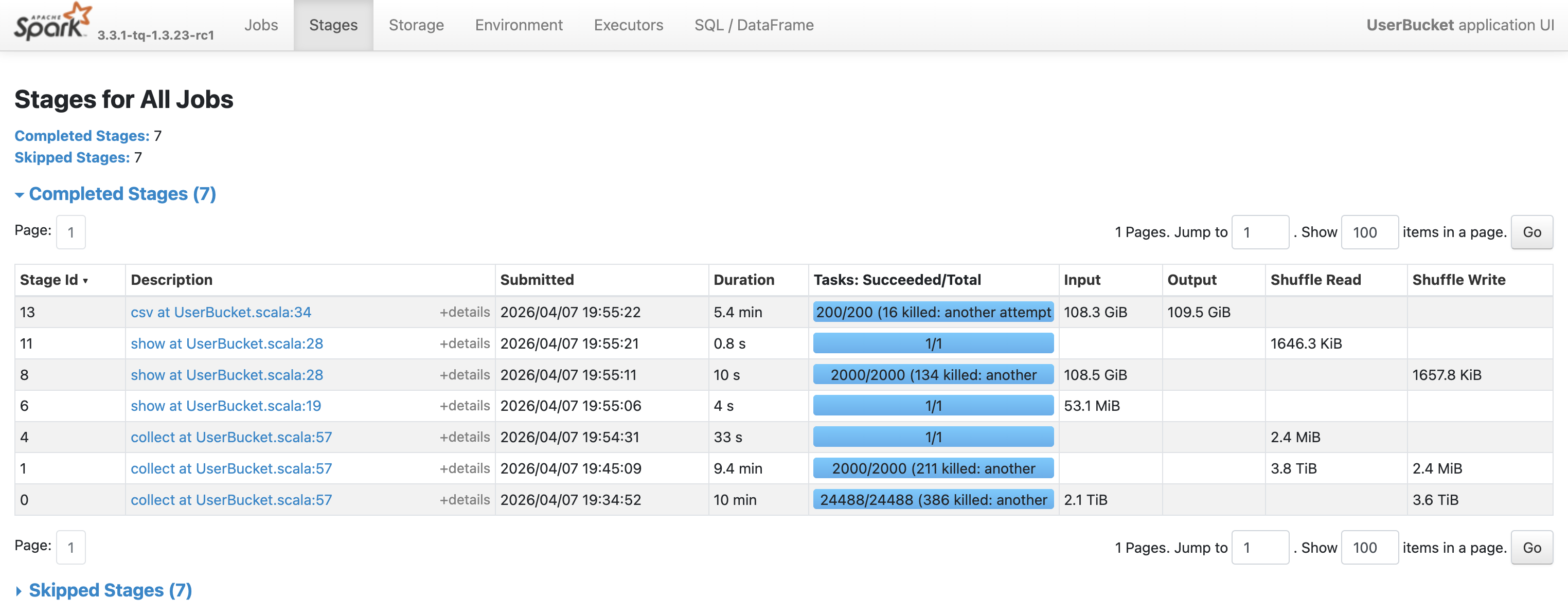
耗时缩短到27 min（计算22 min + 输出5.4 min）。

计算结果中各个桶的cpr顺序正确，请求量大致相等。

calcUserBucket finished, cost 1221.96 seconds
+---------+---------+------------+-----------+-----------+
|bucket_id| user_cnt|     req_cnt|    max_cpr|    min_cpr|
+---------+---------+------------+-----------+-----------+
|       10|331748321|274920287794|   1.0449E8|1402.167424|
|        9|183232702|274650091412|1402.167414|  803.64513|
|        8|146740515|292937877345| 803.645125| 549.270396|
|        7|135683719|282257349368| 549.270386| 388.121402|
|        6|118403632|274375513881|   388.1214| 280.258069|
|        5|105833068|267761199624| 280.258065| 200.627931|
|        4|103250637|281394585299| 200.627929|  133.76862|
|        3| 98452352|283643792147| 133.768618|  77.901462|
|        2| 87066739|252093118582|   77.90146|  34.881892|
|        1|798795286|245856876632|   34.88189|        0.0|
+---------+---------+------------+-----------+-----------+

通过与方法1的精确结果进行比较，可以计算出用户分桶的准确率为2017323519/2112604384=95.5%。这个准确率与采样率有关，采样率越高准确率越高，但计算越慢。

方法3：分区排序

方法1之所以那么慢，是因为排序阶段由单个task完成。可以考虑采用快速排序的思想，将数据集划分为多个分区，分区间有序，然后在各分区内排序，以便利用Spark的并行计算能力。

Spark的键值对RDD支持repartitionAndSortWithinPartitions()操作，能够根据给定的分区器对RDD进行重新分区，并在每个分区内按key进行排序。这种方法比先调用repartition()再在每个分区内排序更高效，因为它可以将排序操作下推到shuffle机制中。

RangePartitioner能够将RDD按照key的范围划分为大致相等的区间。参见 https://zhuanlan.zhihu.com/p/665111208 。

为了使用分区排序，必须将DataFrame转换为RDD[Row]，并以-cpr作为key以便降序排序。repartitionAndSortWithinPartitions()操作生成的RDD是分区间、分区内都有序的。之后依次计算每个分区的累积请求量（相当于手动实现窗口函数），最后转换回DataFrame并计算桶id。完整代码如下：

  
def calcUserBucket(spark: SparkSession, userPosInfo: DataFrame, bucketNum: Int): DataFrame = {
  val userAgg = userPosInfo
    .groupBy("user_id")
    .agg(
      sum("req_cnt").as("req_cnt"),
      sum("cost").as("cost"))
    .filter("req_cnt > 0")
    .withColumn("cpr", expr("cost / req_cnt"))
    .cache()

  val rddWithKey = userAgg.rdd.map(row => (-row.getAs[Double]("cpr"), row))
  val partitionSortedRdd = rddWithKey
    .repartitionAndSortWithinPartitions(new RangePartitioner(1000, rddWithKey))
    .map(_._2)

  val partitionCumReqCnt = partitionSortedRdd
    .mapPartitions(rows => Iterator(rows.map(_.getAs[Long]("req_cnt")).sum))
    .collect()
    .scanLeft(0L)(_ + _)
  val totalReqCnt = partitionCumReqCnt.last

  val cumRatioRdd = partitionSortedRdd.mapPartitionsWithIndex { (idx, rows) =>
    var localCumReqCnt = partitionCumReqCnt(idx)
    rows.map { row =>
      localCumReqCnt += row.getAs[Long]("req_cnt")
      val cumRatio = localCumReqCnt.toDouble / totalReqCnt
      Row.fromSeq(row.toSeq :+ cumRatio)
    }
  }

  val newSchema = StructType(userAgg.schema :+ StructField("cum_ratio", DoubleType))
  spark.createDataFrame(cumRatioRdd, newSchema)
    .withColumn("bucket_id", expr(s"$bucketNum + 1 - ceil(cum_ratio * $bucketNum)")).cache()
}

分桶结果如下，准确率为2112584485/2112604384=99.999%

calcUserBucket finished, cost 13951.86 seconds
+---------+---------+------------+-----------+-----------+
|bucket_id| user_cnt|     req_cnt|    max_cpr|    min_cpr|
+---------+---------+------------+-----------+-----------+
|       10|330282810|272989032912|   1.0449E8|1409.544456|
|        9|182574435|272989105068|1409.544454| 808.294355|
|        8|136727249|272989067180|  808.29435| 566.414343|
|        7|132826920|272989071282|  566.41433| 403.616495|
|        6|119265555|272989045185| 403.616494| 291.970926|
|        5|108953339|272989093350| 291.970925| 208.354515|
|        4|100921987|272989067917| 208.354512| 141.902804|
|        3| 95360210|272989066106| 141.902804|  86.719478|
|        2| 93874745|272989047912|  86.719473|  39.304095|
|        1|808419721|272989095172|  39.304094|        0.0|
+---------+---------+------------+-----------+-----------+

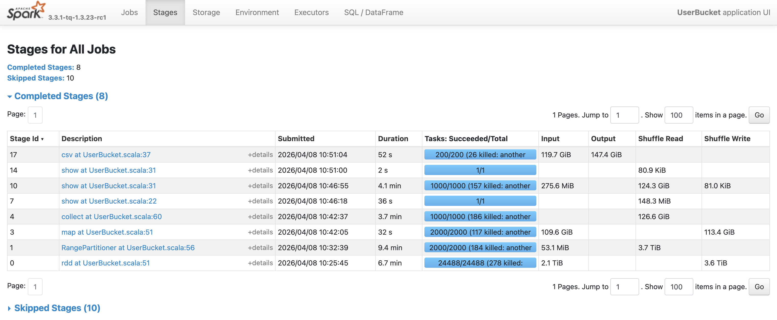
奇怪的是，这次任务花费了7.8 h（计算7.6 h + 输出12 min），反而比全局排序更慢。从Spark UI可以看到，瓶颈在Stage 4和Stage 10，分别耗时3.4 h和3.8 h：

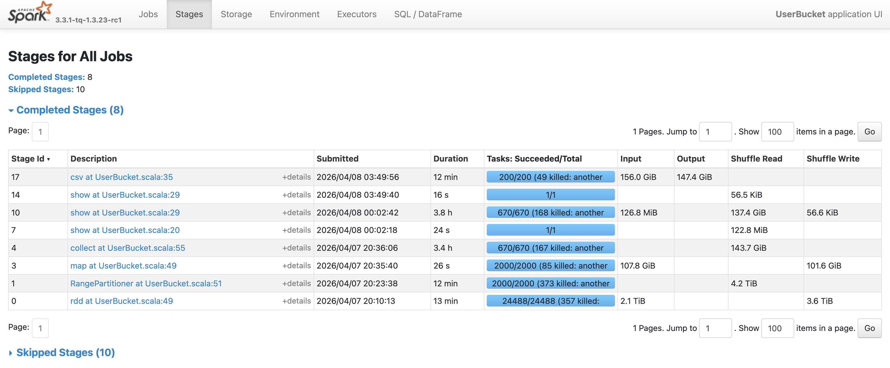
查看这两个阶段内任务的耗时情况，发现红框中任务处理的数据量和耗时远大于其他任务，这是典型的数据倾斜现象。

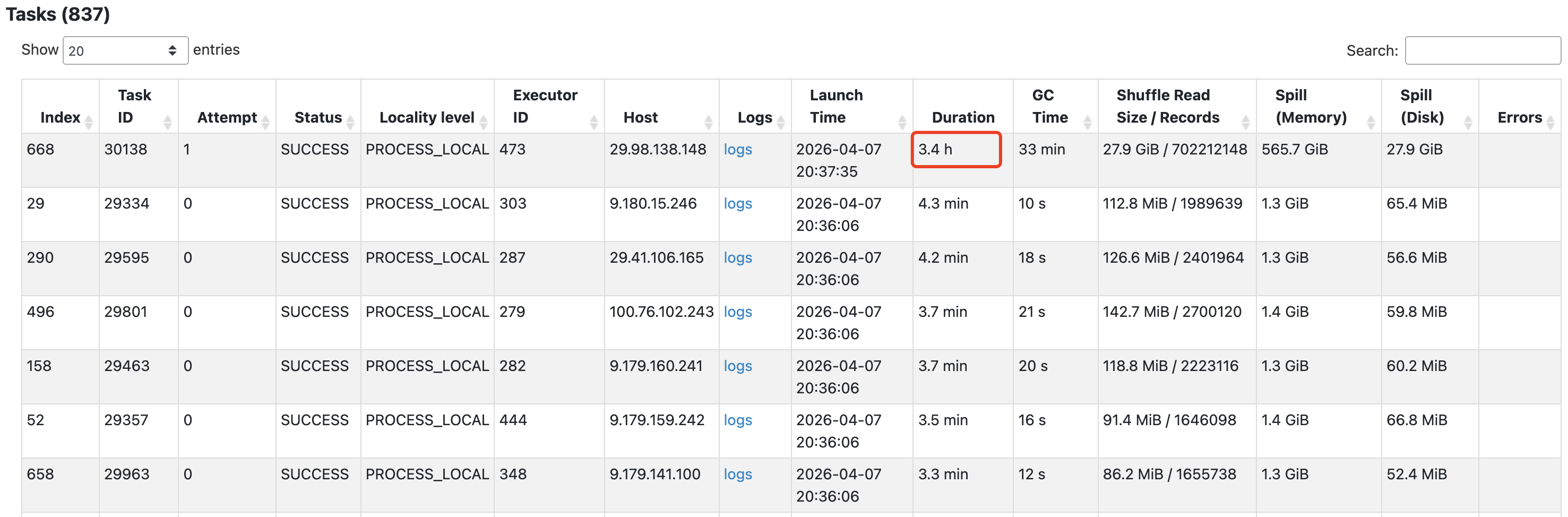
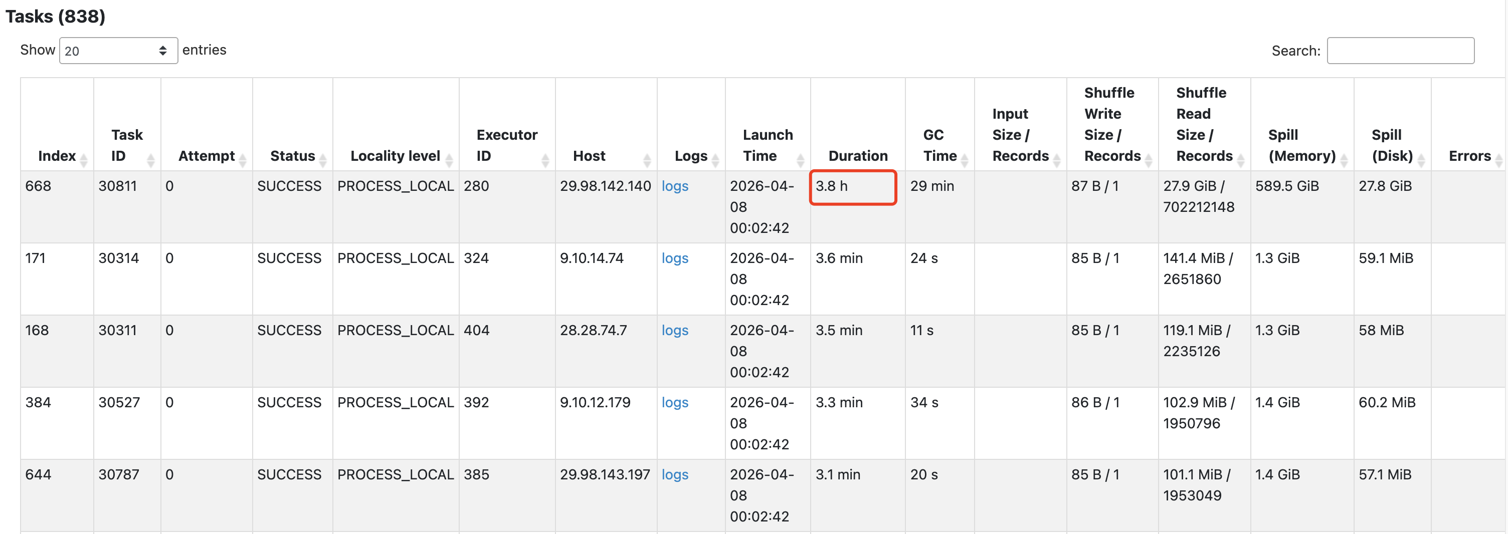
有时还会导致任务反复失败以及executor心跳超时。

为了验证这个问题，统计用户的cpr分布：

cpr	用户数量（亿）
0	7
(0, 10]	0.37
(10, 100]	1.93
(100, 1000]	7.41
(1000, 10000]	3.77
(10000, +∞)	0.5

可以看到，cpr=0的用户占了1/3。RangePartitioner会确保key相等的数据一定在同一个分区，当某个key值的数据量极大时，就会产生严重的数据倾斜。

解决这个问题的常用方法是加盐，即给key添加随机扰动，避免大量数据被划分到同一个分区。

  
val rddWithKey = userAgg.rdd.map { row =>
  val salt = Random.nextDouble() * 1e-6
  (-row.getAs[Double]("cpr") + salt, row)
}

这里选择1e-6是因为相对于cpr值足够小（1桶的cpr上界是39.30），不会影响排序结果，但能够将cpr=0的数据分散到不同分区。

重新运行任务，耗时降至26 min（计算25 min + 输出52 s）。

分桶结果与之前完全相同。

calcUserBucket finished, cost 1275.07 seconds
+---------+---------+------------+-----------+-----------+
|bucket_id| user_cnt|     req_cnt|    max_cpr|    min_cpr|
+---------+---------+------------+-----------+-----------+
|       10|330282810|272989032912|   1.0449E8|1409.544456|
|        9|182574435|272989105068|1409.544454| 808.294355|
|        8|136727249|272989067180|  808.29435| 566.414343|
|        7|132826920|272989071282|  566.41433| 403.616495|
|        6|119265555|272989045185| 403.616494| 291.970926|
|        5|108953339|272989093350| 291.970925| 208.354515|
|        4|100921987|272989067917| 208.354512| 141.902804|
|        3| 95360210|272989066106| 141.902804|  86.719478|
|        2| 93874745|272989047912|  86.719473|  39.304095|
|        1|808419721|272989095172|  39.304094|        0.0|
+---------+---------+------------+-----------+-----------+

分区排序的方法既能加快计算速度，同时又保持了较高的准确率。唯一的缺点是代码实现比较复杂，必须回退到处理RDD[Row]。

总结

下表总结了本文尝试的三种方法的优缺点以及适用场景。

方法	耗时	准确率	优点	缺点	适用场景
全局排序	6.1 h	100%	实现简单，绝对准确	速度太慢	数据量小或对准确性要求高
采样+近似分界点	27 min	95.5%	速度快	准确率较低，与采样率有关	对准确性不敏感，追求速度
分区排序	26 min	99.999%	速度快，准确率高	代码实现较复杂	平衡速度和准确性

Spark

spark data skew

This post is licensed under CC BY 4.0 by the author.

问题定义

方法1：全局排序

方法2：采样+近似分界点

方法3：分区排序

总结

Trending Tags